🦾Build a Python Coding LLM using MLX in Apple Silicon chip

TL;DR

This article is only intended to teach how to implement an LLM architecture from scratch using MLX and train it in a Apple Silicon chip.

Why implement using Apple’s MLX in its Silicon, and not NVIDIA GPU?

As a Mac user, I envy that every people prefers NVIDIA for any work relating to Large Language Model (LLM). This makes the whole ML community constricted to only one GPU vendor (most of the times).

While there are some open source software in this space agnostic to GPUs, many are built around NVIDIA GPUs.

Is it possible to train a Large Language Model possible in Apple Silicon?

Yes and No. This totally depends on the VRAM — the biggest bottleneck for an LLM. In this blog, I will be giving a short brief of how attention mechanisms work and how a langauge model of parameter size ($>300M$) can be trained in an Apple Silicon from scratch using MLX library only.

Attention is all you Need

If you have learnt about machine learning, the chances that you heard about “Attention is all you Need” is higher. This research paper published by scientists at Google Research through Arxiv [paper link] in the year 2017, and it talks about how two blocks essentially help in predicting next words aka tokens.

Note: Word and Token are different here. Token is the right verbalism to use in the context of Large Language Model (LLM).

The original “Attention is All You Need” paper introduced an encoder-decoder architecture for translation tasks. However, GPT uses only the decoder part — this is called a “decoder-only” architecture.

For code generation, we don’t need an encoder because we’re doing autoregressive generation. Since, we are predicting one token at a time based on previous tokens, we don’t need an encoder model to translate between two sequences. The decoder in GPT uses masked self-attention, and each token can only attend to previous tokens, not future ones. This is crucial for autoregressive generation.

After passing through multiple transformer blocks, we use a final linear layer (lm_head) to project from embedding space (d_model dimensions) to vocabulary space (vocab_size dimensions), giving us logits for each possible next token.

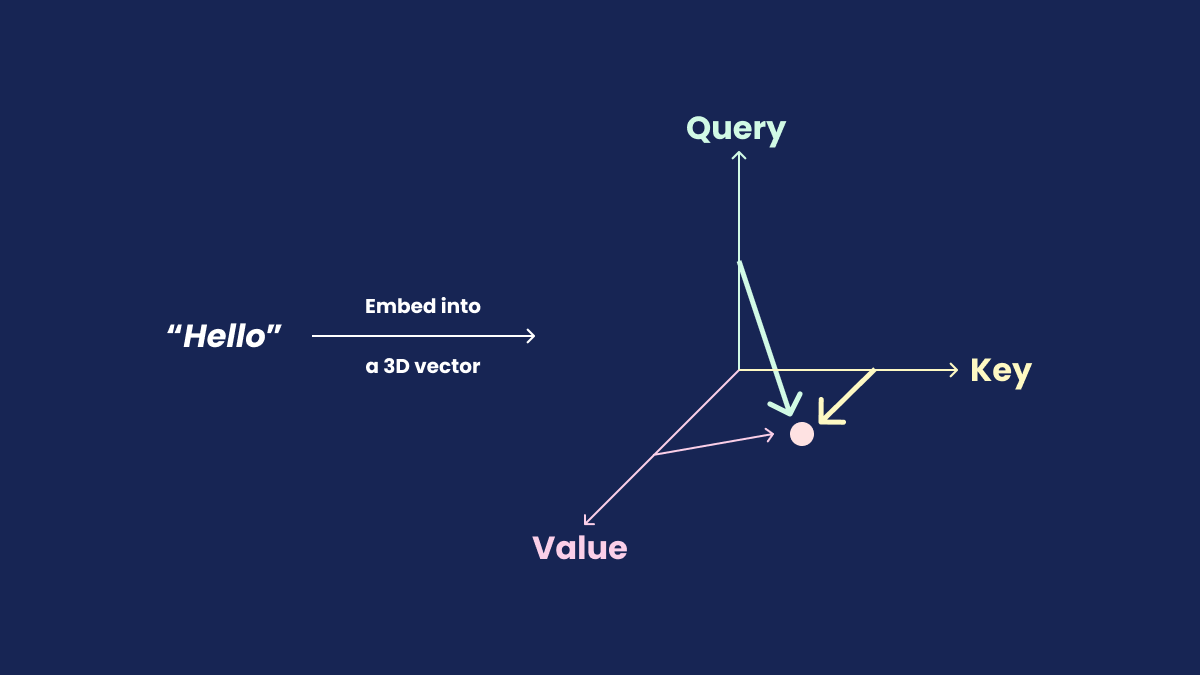
The illustration below depicts a rudimentary function of how the encoder works.

Note: In real world models, Q, K, and V aren’t literally orthogonal or geometric axes. They’re learned projections and can have any orientation in the embedding space.

Text to vector embedding respresented as a 3D space vector

Okay, if it still difficult to grasp how these block work in unison and why this is needed to power an LLM, here’s why: As a human, when someone asks you a question, you think before you answer. Similarly, an LLM needs training data to learn patterns and relationships. Without proper training, the model will generate incorrect outputs. Analogoes to human brain, an LLM is trained on a dataset helping it to predict next set of tokens to answer.

But the real question is: How did scientists at Google Research come up with a solution — Probability! Since computers can only understand binary inputs, texts are converted to vector embeddings (datatype of floating precision numbers), and introduced a probability function to predict the next likely token.

Causal Masking: The Key to Autoregressive Generation

For GPT to work correctly, we need causal masking - ensuring each token can only attend to previous tokens, not future ones. Without this, the model would “cheat” during training by seeing the answer it’s supposed to predict!

We implement this using a lower triangular mask that blocks attention to future positions (using mlx.core.tril API)

Visualising an LLM architecture in Web

There are many websites animating the workflow of attentions and how it enables transformers to predict next likely token in an LLM. Here are my list of favourites:

1. BBYCroft — explaining LLM architecture visually in detail
2. Transformers Explained by Polo Club from Georgia Tech

What is MLX?

MLX is Apple’s answer to JAX — a NumPy-like framework optimized for Apple Silicon’s unified memory architecture, enabling efficient ML training and inference on Mac.

What does an LLM architecture look like?

From the “Attention is all you Need” research paper, we can see how the whole works.

GPT LLM architecture block diagram with decoder sequence only

Image credits: Stack Overflow

The main elements required to build it are:

1. Tokenization
2. Positional Encoding
3. Add and Norm layer(s)
4. Multi-Head attention
5. Feed Forward Network
6. Softmax function

Tokenization and Token Embedding

Apple MLX doesn’t have native support for token embedding like PyTorch’s nn.Embedding [PyTorch (v2.9 stable) API]. Instead of implementing a tokenizer from scratch and training it, we can use a pre-existing model from GPT-2’s tokenizer. This saves us time and suffices the purpose of implementing an LLM from scratch using MLX.

from transformers import AutoTokenizer

# Existing tokenizer to create a new tokenizer model from a dataset
base_tokenizer = AutoTokenizer.from_pretrained("gpt2")
new_tokenizer = base_tokenizer.train_new_from_iterator(raw_dataset_tokenization, vocab_size=52000)

new_tokenizer.save_pretrained("<tokenizer-name>")

Let’s use a dataset from Huggingface to train a GPT model to generate Python code:

# Prerequisites:
# !pip install datasets
# !pip install transformers
from datasets import load_dataset
from transformers import AutoTokenizer


# NOTE: For development purpose, we only use 10,000 rows from the dataset
# Feel free to change this limit
dataset = load_dataset("jtatman/python-code-dataset-500k", split="train[:10_000]")
print(dataset)
# Dataset({
#     features: ['output', 'instruction', 'system'],
#     num_rows: 10000
# })

# To create tokenization, we first create a string with instruction,
#  separated by space, followed by output and <EOS>
# NOTE: <EOS> denotes "(E)nd (O)f (S)equence"
raw_dataset_tokenization = [f"<INSTRUCTION> {data['instruction']} <SEP> <OUTPUT> {data['output']}<EOS>" for data in dataset]
print(len(raw_dataset_tokenization)) # 10000

base_tokenizer = AutoTokenizer.from_pretrained("gpt2")
new_tokenizer = base_tokenizer.train_new_from_iterator(raw_dataset_tokenization, vocab_size=52000)

new_tokenizer.save_pretrained("./data/<...>") # save in folder ./data/<...>
print(new_tokenizer("print hello in python")) # {'input_ids': [518, 6371, 279, 3504], 'attention_mask': [1, 1, 1, 1]}

Now, let’s initialize three classes named TokenEncoding, PositionalEncoding, and TransformerEmbedding. If you go through the code, you will notice that the code looks similar to PyTorch and NumPy implementation.

import mlx.core as mx
import mlx.nn as nn

class TokenEncoding(nn.Module):
    def __init__(self, vocab_size: int, d_model: int):
        super(TokenEncoding, self).__init__()
        self.weight = mx.random.normal((vocab_size, d_model))

    def __call__(self, x: mx.array):
        return mx.take(self.weight, x, axis=0)

class PositionalEncoding(nn.Module):
    def __init__(self, d_model: int, max_len: int):
        super(PositionalEncoding, self).__init__()
        self.pe = mx.zeros((max_len, d_model))
        position = mx.expand_dims(mx.arange(0, max_len), 1)
        div_term = mx.exp(
            mx.arange(0, d_model, 2) *
            -(math.log(10e3) / d_model)
        )

        self.pe[:, 0::2] = mx.sin(position * div_term) # Even dimensions -> use sinusoidal
        self.pe[:, 1::2] = mx.cos(position * div_term) # Odd dimensions -> use cosine
        self.pe = mx.expand_dims(self.pe, 0)

    def __call__(self, x: mx.array):
        seq_len = x.shape[1]

        return x + self.pe[:, :seq_len, :]

class TransformerEmbedding(nn.Module):
    def __init__(self, 
        vocab_size: int,
        d_model: int,
        max_len: int = 5000
    ):
        super(TransformerEmbedding, self).__init__()
        self.token_emb = TokenEncoding(vocab_size, d_model)
        self.pos_emb = PositionalEncoding(d_model, max_len)
        self.scale = math.sqrt(d_model)

    def __call__(self, input_ids, attention_mask: mx.array | None = None):
        embeddings = self.token_emb(input_ids) * self.scale
        embeddings = self.pos_emb(embeddings)
        if attention_mask is not None:
            embeddings = embeddings * mx.expand_dims(attention_mask, -1)
        
        return embeddings

Hence, with TokenEncoding and PositionalEncoding, we can build a tensor to project a 3D vector data in space using the TransformerEmbedding class implementation.

Add and Norm layer

This layer is a residual connection followed by layer normalization; Residual connection was introduced through the ResNet research [Arxiv paper link].

It is used for stablizing the neural network while training. This is a vital layer to train a Large Language Model (LLM).

class AddAndNorm(nn.Module):
    def __init__(self, d_model):
        super(AddAndNorm, self).__init__()
        self.layer_norm = nn.LayerNorm(d_model)

    def __call__(self, x: mx.array, sublayer_out: mx.array):
        return self.layer_norm(x + sublayer_out)

Feed Forward Network

The feed forward network in this architecture is responsible to advance to the next neural network in the layer; helping in predicting the next token from the calculated weights.

Note: We’ll be using ReLu here, but GeLu is highly recommended (available through PyTorch API)

class FeedForwardNetwork(nn.Module):
    def __init__(self, d_model: int, d_ff: int):
        super(FeedForwardNetwork, self).__init__()
        self.W_1 = nn.Linear(d_model, d_ff)
        self.W_2 = nn.Linear(d_ff, d_model)
        self.act = nn.relu

    def __call__(self, x: mx.array):
        return self.W_2(self.act(self.W_1(x)))

Attention Head

This is the main block of an LLM architecture. Here, token is split into 3D space vector as $<Q, K, V>$, or also known as Query, Key, and Value.

class AttentionHead(nn.Module):
    def __init__(self, d_model: int, d_k: int):
        super(AttentionHead, self).__init__()
        self.W_q = nn.Linear(d_model, d_k)
        self.W_k = nn.Linear(d_model, d_k)
        self.W_v = nn.Linear(d_model, d_k)
        self.scale = d_k ** 0.5

    def __call__(self, x: mx.array, attention_mask: mx.array | None = None):
        q = self.W_q(x)
        k = self.W_k(x)
        v = self.W_v(x)
        attention_scores = mx.matmul(q, mx.transpose(k, (0, 2, 1))) / self.scale
        # Apply causal mask
        seq_len = x.shape[1]
        causal_mask = mx.tril(mx.ones((seq_len, seq_len)))
        attention_scores = mx.where(causal_mask, -1e9, attention_scores)

        if attention_mask is not None:
            attention_scores = mx.where(attention_mask, attention_scores, -1e9)
        attention_weights = mx.softmax(attention_scores, axis=-1)

        return mx.matmul(attention_weights, v)

This block follows the illustration from the “Attention is all you Need” research paper.

This is Scaled Dot-Product Attention (similar to Attention Head) along with Multi-Head Attention

Image credits: Attention is all you Need

AttentionHead is similar to the illustration, but the key difference is that AttentionHead class implements Attention with linear passes masks per 3D space projection and returns the matrix multiplication of it. This allows us to create a Multi-head without hassle.

MultiHeadAttention class comprises of multiple AttentionHead, and is responsible to return each token’s projection in 3D space as a tensor.

class MultiHeadAttention(nn.Module):
    def __init__(self, d_model: int, num_heads: int = 8):
        super(MultiHeadAttention, self).__init__()
        self.num_heads = num_heads
        self.d_k = d_model // num_heads
        for i in range(num_heads):
            setattr(self, f"head_{i}", AttentionHead(d_model, self.d_k))

        self.W_o = nn.Linear(d_model, d_model)

    def __call__(self, x: mx.array, attention_mask: mx.array | None = None):
        head_outputs = []
        for i in range(self.num_heads):
            head = getattr(self, f"head_{i}")
            head_outputs.append(head(x, attention_mask))
        concat = mx.concatenate(head_outputs, axis=-1)

        return self.W_o(concat)

Transformer

Once these are done, we can fix these blocks together like a lego block set to train an LLM.

class Transformer(nn.Module):
    def __init__(self, d_model: int, num_heads: int, d_ff: int):
        super(Transformer, self).__init__()
        self.attention = MultiHeadAttention(d_model, num_heads)
        self.add_norm1 = AddAndNorm(d_model)

        self.ffn = FeedForwardNetwork(d_model, d_ff)
        self.add_norm2 = AddAndNorm(d_model)

    def __call__(self, x: mx.array, attention_mask: mx.array | None = None):
        attention_output = self.attention(x, attention_mask)
        x = self.add_norm1(x, attention_output)

        ffn_output = self.ffn(x)
        x = self.add_norm2(x, ffn_output)
        return x

Final Verdict

With these blocks, it builds a transformer architecture; A decoder class has been implemented, and available in my repository [link] — this will contain brief detail into how to use/train/test your large language model.

After training, the model on quick inference would generate like this (not a near-pefect model):

This would be a disaster in production xD

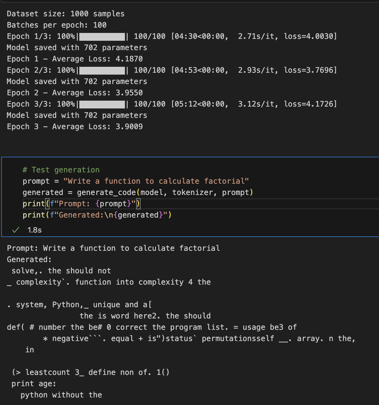
Note: “702 parameters” are the total flattened parameters after training and saving the model — not to be confuse with model parameter size.

Upcoming Steps

• The code must be refined to run in inference mode, and convert from safetensors to GGUF format.
• Fine-tuning with better dataset to enhance code generation accuracy by implementing with plain MLX.